One of the benefits of kinetic Monte Carlo is that it coarse-grains physical space: the reacting molecules are no longer moving and interacting in the 3D space but on a lattice. Thus, diffusion, for instance, is not captured as a continuous (x,y,z)-trajectory but rather as a transition whereby a molecule hops from one site of the lattice to another. Choosing how to map a catalytic surface onto a lattice is relatively simple, but one has to make some decisions that may be important in correctly capturing the relevant physics. This tutorial provides guidance on this matter and explains how to set up the input for a periodic lattice in Zacros. As a working example we will consider a FCC(100) surface.
Within the Graph-Theoretical KMC framework, a lattice is a collection of connected sites. Each site can be of a particular type, making it possible to represent for instance, the atop, bridge, and hollow sites of an FCC metal surface. The information about a periodic lattice is therefore “encoded” in the sites contained unit cell and the connectivity of these sites within the cell, as well as the sites of the neighbouring cells. In the following, we will explain how one can set up the lattice_input.dat in Zacros for a FCC(100) surface input for files.
Part 1: Preliminary considerations
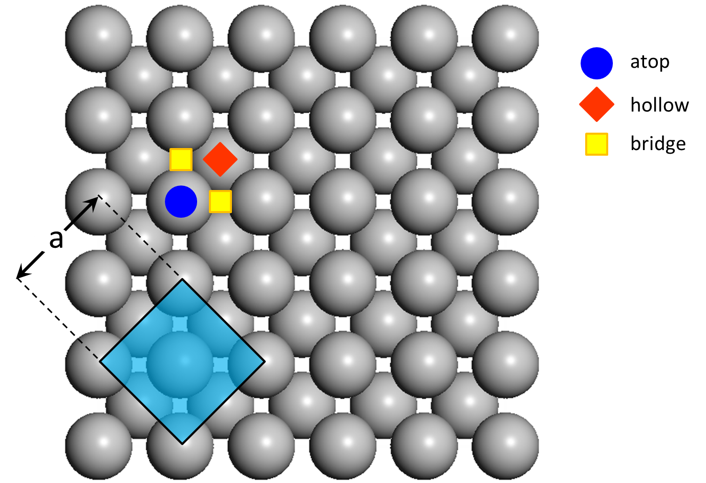
In the (100) surface of an FCC metal, each atom is surrounded by four neighbouring atoms and one can discern three site types: atop, 2-fold bridge and 4-fold hollow. The surface is shown schematically below, highlighting also the unit cell of the FCC crystal and the lattice constant, which for the case of Pd for example is a = 3.8907 Å.
In order to create a lattice that will be appropriate for our simulations and will not contain unecessary detail that may hamper the simulation, we need to answer the following questions:
- Which sites are important?
Density functional theory calculations can reveal the sites which the molecules of interest bind to most strongly. If the most stable configurations of our reactant and intermediate species bind to say the atop and hollow sites, and binding to the bridge site is much weaker, we only need to consider the former two sites, i.e. we can neglect the bridge site as irrelevant.
Of course, when comparing binding energies on different sites to determine the most stable configurations, we have to keep in mind that depending on the temperature of the simulation, we may or may not be able to safely neglect some configurations. In particular, a difference of 0.05 eV between the binding energies of a species on two site types may be significant at low temperatures, and therefore considering only the most site may be enough. At high temperatures, however, the lower binding energy site may be highly populated as well, which would necessitate taking into account both sites in the lattice definition.
- How to connect the sites?
Site connectivity in the lattice is determined by the elementary reaction events we need to model, as well as the energetic interactions between adsorbed species. If you are unfamiliar with these concepts, please refer to the tutorials Ziff-Gulari-Barshad Model in Zacros and Cluster Expansion for Oxygen on Pt(111). The rule is that if two sites participate in an elementary reaction or an energetic interaction pattern, then they have to be connected, either directly, or indirectly via one or more other sites. This enables the Graph-Theoretical KMC algorithm to detect the patterns efficiently by solving subgraph isomorphism problem. For instance, if a diffusional hop can happen from a hollow site to another, these sites must be connected in our lattice.
Let us assume that for our purposes it is enough to model the atop and 4-fold hollow sites only. Also, let us decide to model all three possible links between these two site types: atop-atop, hollow-hollow and atop-hollow. In the following section we will discuss how to draw a lattice picture that can be translated to Zacros input in a straightforward way.
Part 2: Drawing the lattice
To make a drawing of the lattice that can be directly translated to Zacros one can follow these steps:
- Draw the unit cell with all sites therein.
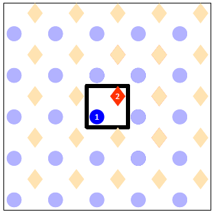
It is advisable to use different markers or colours to denote the different site types. For our lattice, the drawing after this step would contain the square with the thick line and the sites with the vivid colours as displayed below. The blue circles denote the atop sites and the orange diamonds the 4-fold hollow. To show how the lattice would look like when this unit cell is tiled on the plane we have also drawn many more sites around the unit cell in pale colours.

- Number all the sites within the unit cell.
We have two sites inside our unit cell, which will be numbered as 1 for the atop and 2 for the hollow. If there were more than one sites of the same type, for instance two atop sites, we would have to assign a different number to each site, so we could have site number 1 being atop, site number 2 being atop, site number 3 being hollow etc. At the end of this step our drawing looks like the following:
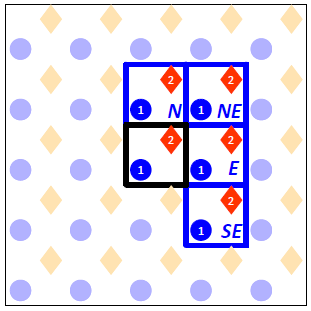
- Draw periodic images of the unit cell clockwise starting from the North neighbour (marked N) to the SouthEast neighbroud (marked SE).
This is in preparation to the next step, in which we will be drawing the links between the connected sites. Note that due to symmetry we do not need to specify any links with the remaining 4 neighbours (South to NorthWest). For instance, if site 1 at the Central cell neighbours with site 2 at the North cell, it follows that site 2 at the Central cell will neighbour with site 1 at the South cell. At the end of this step our drawing looks like this:
- Mark all links between the sites of the central cell with the sites of the neighbouring cells.
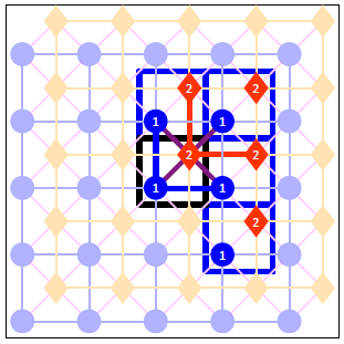
In our case we have a total of 8 links: the atop site of the Central cell connects with the atop sites of the North and East neighbours; similarly the hollow site of the Central cell connects with the hollow sites of the North and East neighbours. Also, the hollow site at the Central cell is connected with the atop site in that same cell and the atop sites of three neighbours. At the end of this step our drawing looks as shown below (note that we have dropped the designations N, NE, E and SE of the four neighbouring cells to avoid cluttering the picture):
In the next section we will see how the above figure can be translated to a lattice_input.dat file that can be parsed by Zacros.
Part 3: Generating the lattice input file
The lattice input file starts with the keyword lattice followed by one of: default, periodic_cell or explicit. We have already seen the use of a default lattice in tutorial Ziff-Gulari-Barshad Model in Zacros. Here we will focus on the second type of lattice defined as a periodic tiling of a unit cell. So in our input file the first line will be:
lattice periodic_cell
The next few lines of the input file define the two unit cell vectors, a and b. The keyword cell_vectors is used followed by two lines, each of which contains the x and y components of each vector. In our case the unit cell vectors are the cartesian unit vectors times a lattice constant. For the case of Pd, the lattice constant of the cubit unit cell of the crystal is 3.8907 Å and the unit cell for the surface lattice will have a lattice constant of 3.8907×√2/2.
cell_vectors
   2.751140353562500 0.000000000000000 # x and y components of a
   0.000000000000000 2.751140353562500 # x and y components of b
We will also have to define how big the KMC simulation lattice will be. We will therefore have to tell Zacros how many times do we want to tile the unit cell along the directions of the vectors a and b. Let's say we want a 50×50 lattice; then we have to use the expression:
repeat_cell 50 50
Next, we will have to define the different site types that can appear in the unit cell, which in our case are atop and hollow. We therefore need to first tell Zacros that there are two different site types and then define the names we will use to refer to them:
n_site_types      2
site_type_names   top hol
These site type names (top, hol) can subsequently be used in the definition of energetic interaction or elementary reaction patterns, enabling us for instance to define different adsorption energies on different sites, or different activation energies for the same elementary step when it occurs on different site types (or combinations or site types for multi-site events).
We are now ready to define the lattice structure, which involves three things: (1) defining the type of each of the two sites contained in the unit cell, (2) defining the coordinates of each site, and (3) specifying the neighboring structure of the lattice. Let us bring back the drawing we made in the previous section of the tutorial to make it apparent how it helps us with these tasks:
The definition of the site types and the coordinates is easy: focus on the central cell, and for each of the sites that we have therein numbered as 1, 2, ... (here we have only two), list the corresponding site type. In our case we have top hol, since the first type is atop and the second hollow. In Zacros parlance:
n_cell_sites      2
site_types        top hol
Equally well we could have written site_types 1 2 in the second line (i.e. use the site type index instead of the corresponding name).
The coordinates of each site are defined as fractional (rather than Cartesian) coordinates, using the keyword site_coordinates followed by as many lines as the number of sites in the unit cell. Each line gives the a and b fractions coordinates of the corresponding site, such that if λ and μ are the fractional coordinates, the cartesian coordinates of the site (in the central unit cell) are (x,y) = λ a + μ b.
site_coordinates
   0.250000000000000 0.250000000000000 # a, b frac. coords of 1st site
   0.750000000000000 0.750000000000000 # a, b frac. coords of 2nd site
The final thing we need to define is the links between neighbouring sites, which is done within a neighboring_structure ... end_neighboring_structure block. To this end, we look at the drawing above, which highlights the links between any site in the central cell with any site either in the central cell or any of the four neighboring cells. Thus, links between sites that both belong to neighboring cells are excluded. For each of the highlighted links we write one line in the neighboring_structure ... end_neighboring_structure block containing the indices of the two neighboring sites separated by a dash and followed by one of the following keywords: self if both sites are in the central cell, north,northeast,east,southeast if the second site is in the north, northeast, east or southeast neighboring cells, respectively. Note that in the latter four cases the second index must correspond to the site in the neighbouring cell. In the first case, the order of the indexes of the cells does not matter. The eight links of the drawing above are thus translated in the following Zacros instructions:
neighboring_structure
   1-2 self
   1-1 north
   1-1 east
   2-1 north
   2-1 northeast
   2-1 east
   2-2 north
   2-2 east
end_neighboring_structure
Note that the order in which the neighbouring instructions appear within the block does not matter.