Ziff, Gulari and Barshad were the first to demonstrate kinetic phase transitions in a conceptual model for CO oxidation on the surface of a heterogeneous catalyst [R. M. Ziff, E. Gulari, Y. Barshad (1986) Phys. Rev. Lett. 56: 2553]. Using a mechanism that includes the non-dissociative adsorption of CO, the dissociative adsorption of O2, and the fast CO oxidation reaction Ziff et al., found a second order phase transition from an O-poisoned regime to a reactive regime, and a first order transition from the reactive to the CO-poisoned regime. Such a model can be easily set up in Zacros: this tutorial explains how to create the necessary input files.
The conceptual CO oxidation model by Ziff, Gulari and Barshad (ZGB) served as the first demonstration of kinetic phase transitions in heterogeneous catalytic systems.1 The model includes 3 irreversible events: non-dissociative adsorption of CO, dissociative adsorption of O2, and fast reaction between an O adatom and a CO adsorbate. Such a model can be easily set up in Zacros. In this tutorial we will discuss how to create the input files for such a simulation. By changing the molar fractions of the CO and O2 species, one can reproduce the phase diagram of the original paper by Ziff et al.1
Part 1: General settings
The simulation_input.dat file contains information about the gas and adsorbed species, the conditions of the simulation, as well as instructions about sampling over the course of the simulation and stopping criteria. One can also set the seed of the random number generator, so that different runs with the same seed produce the same results. The random seed is set as:
random_seed 953129
The conditions of the simulation are specified by expressions such as:
temperature               500.0
pressure                  1.0
Next comes the information about the gas phase species. In our simulation we have three gas phase species, CO, O2 and CO2. We have to specify the energies, molar fractions and molecular weights (the molecular weights are not used currently in the simulation, the corresponding keyword is there for future development purposes).
n_gas_species             3
gas_specs_names           CO        O2       CO2
gas_energies              0.000     0.000    -2.337 # in eV
gas_molec_weights        28.0102   31.9989   44.0096
gas_molar_fracs            0.450    0.550     0.000
The names of species can be whatever the user wants. It helps to use names indicating chemical formulas for simple species. Also, as a convention, the * character should be reserved to only adsorbed species, as discussed below. The information about the gas energies can be found by density functional theory (DFT) calculations (note that comments in the input files are preceded by the character #). Zacros uses this information to compute the reaction energy (ΔErxn) and subsequently the activation energy via Brønsted-Evans-Polanyi relations. In the context of the ZGB model, these energies are not important, since the rate constants of the elementary events are given explicitly, so we will take all activation energies equal to 0. Consequently, the actual simulation temperature defined above, will not change the simulation results. The molar fractions are important though, as they determine the relative frequency of CO versus O2 adsorption, which in turn shapes system behaviour (regimes where poisoning versus sustained reactivity is observed).
The specification of adsorbed species is a bit simpler. Here we have only 2 adsorbates, CO and O. In naming these species, we conventionally use one or more * characters in the end of the name, to indicate how many sites this species is bound to. For instance, a monodentate species would be A*, a bidentate B** etc. In our case:
n_surf_species            2
surf_specs_names          CO* O*
surf_specs_dent           1   1
The last keyword surf_specs_dent, indicates the denticity of each species, namely the number of sites occupied. In our case we have only monodentate species.
The sampling behaviour of the programme is controlled by the keywords: snapshots, process_statistics, species_numbers. Keyword snapshots controls how often Zacros saves lattice configurations to the history_output.dat file, process_statistics pertains to the statistics of elementary event occurrence saved in file procstat_output.txt, and species_numbers pertains to the numbers of gas species produced or consumed, as well as the number of adsorbed molecules/atoms found on the lattice, which are reported in file specnum_output.txt. Each of these keywords can be followed by the expression on event, in which case, Zacros logs down a new entry in the corresponding file every time an elementary event is executed. On the other hand the keywords can be followed by the expression on time and a real number, in which case saving occurs after a fixed time interval Δt. The sampling modes or the Δts for each output file need not be the same, for instance, one might want to save snapshots every 1 s of simulated time, but report species numbers at every event occurrence. In our case, we will use the following options:
snapshots                 on time 5.e-1
process_statistics        on time 1.e-2
species_numbers           on time 1.e-2
Note that too frequent sampling can result in huge output files, so the on event sampling mode should typically be restricted to short exploratory simulations, rather than production runs.
The KMC simulation can stop when a fixed number of events has been simulated, or when the simulation time has reached a given value. Thus, stopping criteria can be defined by the keywords max_steps or max_time, which can be followed by an integer or real, respectively; or by the keyword infinity. The latter immediately sets the maximum number of steps or the maximum time, to the biggest allowed value (about 9.2e+18 steps, or 1.8e+308 units of simulated time on GNU fortran). Here we will use:
max_steps                 infinity
max_time                  25.0
Another stopping criterion has to do with the actual (real) time the simulation has run for, and may come in handy when running in computational clusters with walltimes. The keyword is walltime, and is followed by an integer specifying the number of seconds the simulation is allowed to run. In the end of the simulation, Zacros will write a restart.inf file (unless the keyword no_restart appears in simulation_input.dat), and exit normally. If Zacros is invoked from a directory where a restart.inf file appears, it will disregard any input files (*_input.dat) and attempt to resume the simulation saved in the restart file. In our example here, we will specify a walltime of 1 hour:
wall_time 3600 # in seconds
The simulation_input.dat file ends with the keyword finish.
Download simulation_input.dat.
Part 2: Lattice structure
The original ZGB model was simulated on a rectangular lattice (coordination number 4). Zacros has this structure implemented as a default lattice, along with a hexagonal and a triangular lattice (coordination numbers 6 and 3). To use one of the default lattices, one has to start the lattice_input.dat with the keywords:
lattice default_choice
The rectangular lattice is then invoked by the keyword rectangular_periodic, which is followed by one real, specifying the lattice constant, and two integers, specifying the size of the lattice. In the following, we construct a 50×50 lattice with lattice constant equal to 1:
rectangular_periodic 1.0 50 50
Thus, the full contents of the lattice_input.dat file are as follows:
lattice default_choice
rectangular_periodic  1.0 50 50
end_lattice
Part 3: Energetics model
The specification of an energetics model is very important in detailed KMC simulations, as it captures the adsorbate-adsorbate lateral interactions responsible for ordering in the adsorbate overlayer. Lateral interactions also affect the activation barriers of elementary events, by stabilising or destabilising the initial, transition, or final state of the event.
The ZGB model does not include lateral interactions between adsorbates and the rates of events are explicitly defined (so activation energies will be taken as 0). We will, however, discuss, for the sake of completeness how to set up a simple model for the energetics, including only the binding energies of individual adsorbates (no interactions). We will assume a binding energy of 1.3 eV for CO and 2.3 for O.
Zacros implements a general cluster-expansion Hamiltonian approach for the energetics. In this approach, the energy of a given configuration is computed by summing up single-body contributions, as well as two-body, three-body etc. interaction terms. Thus, we have to define the individual patterns contributing to the overall energy, and the individual energy contribution of each pattern. This is done in the energetics_input.dat file which starts with keyword energetics, followed by one or more blocks of instructions contained within keywords cluster … end_cluster. The parsing of the file finished when Zacros encounters the keyword end_energetics.
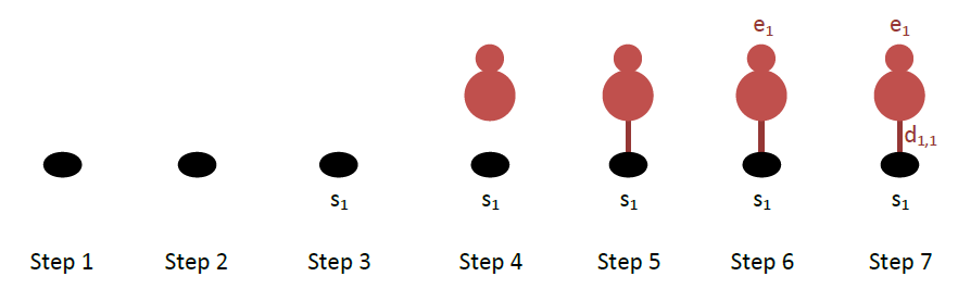
To define correctly the patterns in Zacros, it is often helpful to make a schematic of the binding configuration wherein you clearly number the sites, adsorbate molecules and dentates thereof. This drawing process can be accomplished by following these steps:
- Draw all the sites involved in the pattern.
- If more than one sites are involved, draw all the links between the sites indicating which sites are neighbours.
- Number all the sites in the pattern, as s1, s2,…
- Draw all the adsorbate entities participating on the pattern, clearly indicating the species type for each entity.
- Draw the bonds between adsorbates and sites, to clearly indicate which adsorbate occupies which site (or sites, if there are multidentate adsorbates).
- Number all adsorbates (entities) as e1, e2,…
- Number all dentates as d1,1, d1,2, …, d2,1, d2,2,… The first index in this numbering system is the entity number, and the second is the dentate number.
Let us do this for CO: this molecule binds to a single site. The drawings per step are shown below:
The Zacros input for the CO binding pattern starts with the keyword cluster followed by the name of the pattern:
cluster CO_point
Then, the number of sites involved is defined as follows:
sites 1
In this case we have only one site, so there are no links between sites. If we had 2 or more sites, we would have to define the neighbouring structure of the pattern using the keyword neighboring, which however in our case is omitted.
The most important part of the cluster definition is the description of the occupancies of the sites, which is done with the lattice_state keyword. This keyword is followed by as many lines of input as the number of sites in the pattern (in this case only one). Each line contains three words: the first is the number of the entity/adsorbate occupying the corresponding site, the second is the species name occupying that site, and the last word is the dentate number with which the entity binds to that site. In our case (see above figure), site number 1 is occupied by dentate 1 of entity number 1, which is a CO*. Therefore:
lattice_state
  1 CO*  1
The last two things we need to define here are the graph multiplicity and the energy contribution of the cluster (also referred to as effective cluster interaction). The multiplicity is defined by the optional keyword graph_multiplicity, whereas the energy contribution is specified with the keyword cluster_eng. If graph_multiplicity is absent, a default value of 1 is used for the multiplicity. The latter exists for cross-compatibility with other KMC software codes: when Zacros detects this pattern on the lattice, it will add a contribution of cluster equal to the cluster energy divided by the multiplicity. This is useful, for instance, in the case of a symmetric pairwise pattern, which will be detected twice by the Zacros algorithm. A multiplicity of 2 will correct for this double-counting. In our case, we have a single site pattern so things are rather simple:
graph_multiplicity  1
cluster_eng        -1.3
The cluster specification block ends with the keyword end_cluster.
Similarly, the corresponding block for the adsorbed O cluster is:
cluster O_point
  sites 1
  lattice_state
    1 O*  1
  graph_multiplicity  1
  cluster_eng        -2.3
end_cluster
Download energetics_input.dat.
Part 4: Reaction mechanism
The reaction mechanism is described in the mechanism_input.dat file. The file starts with the keyword mechanism, and ends with end_mechanism. The contents of the file consist of blocks starting with keyword step (for irreversible elementary steps) or reversible_step (for reversible elementary steps) and ending with end_step, or end_reversible_step, respectively. It is generally recommended to use only reversible steps in KMC simulations otherwise the simulation may violate detailed balance and thermodynamic consistency. For this tutorial we are implementing the ZGB model which is a prototypical irreversible model, so we will only use step … end_step blocks.
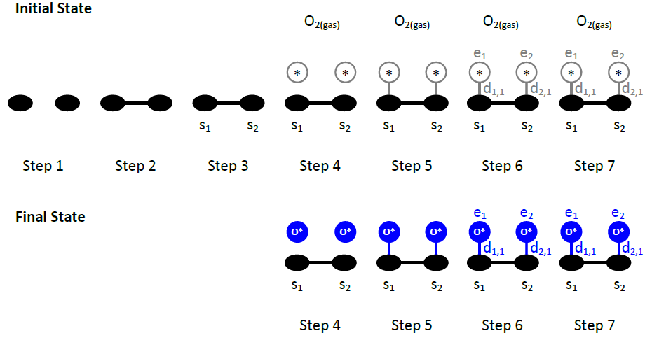
The way one defines the initial and final states of the elementary steps is very similar to the definition of the lattice state in energetic patterns. Thus, to correctly define elementary steps, one can draw pictures of the initial and final states following steps similar to 1-7 outlined in the previous section:
- Draw all the sites involved in the initial state of the elementary event.
- If more than one sites are involved, draw all the links between the sites indicating which sites are neighbours.
- Number all the sites in the pattern, as s1, s2,…
- Draw all the gas species and adsorbate entities participating on the pattern, clearly indicating the species type for each entity. An empty site is assumed to be a site occupied by a “vacancy” pseudo-species.
- Draw the bonds between adsorbates and sites, to clearly indicate which adsorbate occupies which site (or sites, if there are multidentate adsorbates).
- Number all adsorbates (entities) as e1, e2,…
- Number all dentates as d1,1, d1,2, …, d2,1, d2,2,… The first index in this numbering system is the entity number, and the second is the dentate number.
- Repeat steps 4-7 for the final state of the pattern, using the numbering of the sites consistently in the initial and final states of the pattern.
As an example we will demonstrate these pictures for the O2 dissociative adsorption event:
The Zacros instructions for this patter are as follows:
step O2_adsorption
for the definition of the name of the event.
The following line defines the gas phase reactants or products: the keyword gas_reacs_prods can be followed by an arbitrary number of pairs of a gas species name and a stoichiometric coefficient. The latter can be negative, defining a gas phase reactant, or positive defining a product. In our case, an O2 gas molecule is removed upon adsorption.
gas_reacs_prods O2 -1
The next two lines indicate that there are 2 sites involved in this event, which have to be nearest neighbours:
  sites 2
  neighboring 1-2
In the initial state, we have two empty sites on the lattice. Thus, both sites are “occupied” by the vacant species, denoted by the reserved name *. The description of this initial state consists of the keyword initial, followed by 2 lines of 3 words, the 1st line corresponding to site 1 and the 2nd to site 2:
  initial
    1 *     1
    2 *     1
Note that we are consistent with the numbering of the figure above: the first (second) site is occupied by the first (second) entity. The entity numbering makes each line unique in a state specification. Having one or more lines with the exact same information within a state specification (either initial or final) is invalid and will result in an error.
In the final configuration, there are two O adatoms. Consistent with the figure above, we write:
  final
    1 O*    1
    2 O*    1
Further, we have to define a pre-exponential and an activation energy for this event:
  pre_expon  2.5
  activ_eng  0.0
With an activation energy of 0 eV, the kinetic constant of this event is always equal to the pre-exponential value.
Finally, the block ends with the end_step keyword.
The blocks for the CO adsorption and the CO oxidation steps are shown below, followed by the Zacros input for these two events:
step CO_adsorption
  gas_reacs_prods  CO -1
  sites 1
  initial
    1 *     1
  final
    1 CO*   1
  pre_expon 10.0
  activ_eng  0.0
end_step
step CO_oxidation
  gas_reacs_prods  CO2 1
  sites 2
  neighboring 1-2
  initial
    1 CO*  1
    2 O*   1
  final
    1 *    1
    2 *    1
  pre_expon  1.e+20
  activ_eng  0.0
end_step
With regard to the rate parameters for the elementary events, since the original ZGB implementation uses a null-event type of approach, we need to properly choose our kinetic constants to simulate the same behaviour. Thus, the CO oxidation event rate was taken as very high, since in the original ZGB model this event happens immediately when a CO-O pair is formed. The CO adsorption rate pre-exponential was arbitrarily taken as 10 bar-1s-1. Thus, if the partial pressure of CO in the gas phase is 0.45 (see part 1: Simulation setup) the rate will be 4.5 s-1. The O2 adsorption pre-exponential was chosen to be ¼ that of CO: this way, because of the coordination number 4 of the lattice, for every empty site therein, the maximum O2 adsorption rate can be 10 bar-1s-1, when all neighbouring sites are vacant. This setup mimics the null-event approach by Ziff, Gulari and Barshad, wherein for equimolar CO:O2 mixture, an empty lattice has equal probability of being picked for a CO or O2 adsorption event, and the success of an O2 adsorption trial is subsequently determined by looking at the neighbouring sites.
References
- R. M. Ziff, E. Gulari and Y. Barshad (1986), "Kinetic phase transitions in an irreversible surface-reaction model", Phys. Rev. Lett. 56: 2553-2556 (doi: 10.1103/PhysRevLett.56.2553)